本文介绍ggplot2中stat_xxx()相关的设置。
使用ggplot2绘制图表时,涉及统计变换时,这时stat_xxx()函数就派上用场了。统计转换函数是在数据被绘制出来之前对数据进行聚合和其他计算。
常用的stat_xxx()函数有:stat_xxx()确定了数据的计算方法。因此,一个stat函数必须与一个geom()函数相对应才能进行计算。stat_与geom在一定程度上可以互换。
如图: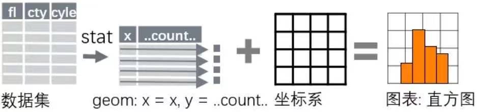
stat_smooth()、stat_bin()、stat_ecdf()、stat_count()、stat_density()、stat_function、stat_summray()等等。
1. stat_summary()
假定我们有一组数据,现在想画一个柱状图,一个柱子代表每一组group,柱子的高度代表的score的均值,这很容易搞定,但是如果我们想要加误差棒呢?我们需要再次整理数据,然后传递给ggplot,整合两个数据,一个用于绘制柱状图,一个用于绘制误差棒。
1 | simple_data_bar <- simple_data %>% |
如果使用stat_summary()函数,很简单就可以实现:
1 | simple_data %>% |
stat_**()函数可以将数据进行内部的统计转换,传递给ggplot()进行画图,因此不需要重新做一个dataframe,简单方便。
例如:
1 | ggplot(df,aes(x,y))+ |
上述例子里,stat_summary()对每一个x,计算y的均值,并在散点图上添加一个均值(白色点)。
stat_summary()适用的几何形状:geom_errorbar()、geom_pointrange()、geom_linerange()、geom_crossbar()、geom_point()。
1 | ggplot(iris,aes(x=Species,y=Sepal.Length))+ |
stat_summary()中函数可以是自定义函数。例如:
1 | my_fun <- function(x){ |
stat_summary()也可以添加文本,geom换成text即可。
2. stat_smooth()
stat_summary()函数用于(为scatter plot)生成拟合曲线。例如,生成回归曲线,se=FALSE生成的图片不包含置信区间。
适用几何形状:geom_smmooth、geom_line()、geom_point()。
1 | ggplot(mtcars,aes(x=mpg,y=disp))+ |
3. stat_bin()
stat_bin()函数对x根据每个bin进行计数。适用的几何形状:geom_bar()、geom_histogram()、geom_freqpoly()。
1 | ggplot(mtcars,aes(x=mpg))+ |
1 | ggplot(mtcars,aes(x=mpg))+ |
上述两个得到的图是一样的。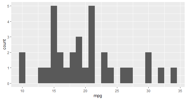
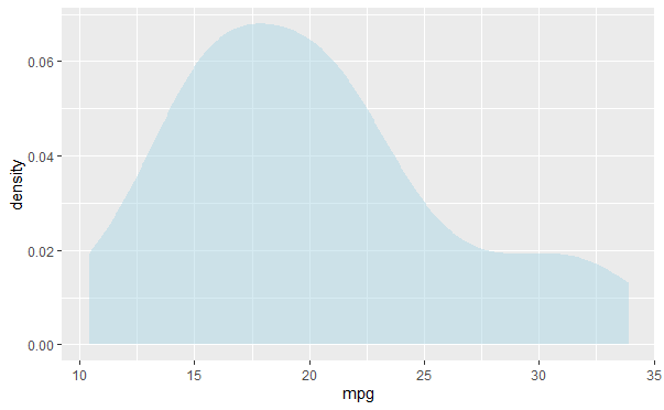
4. stat_density()
stat_density()对一个连续的变量,生成一个density plot。
1 | ggplot(mtcars,aes(mpg))+ |
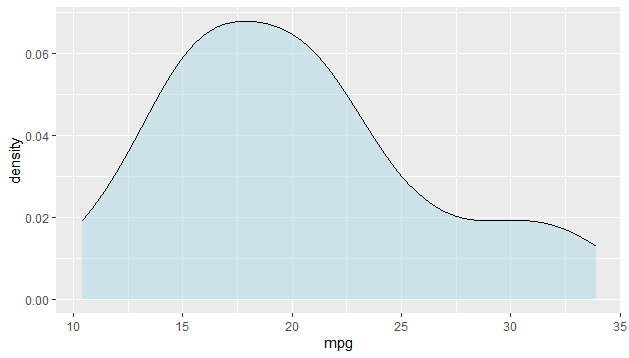
1 | ggplot(mtcars,aes(mpg))+ |
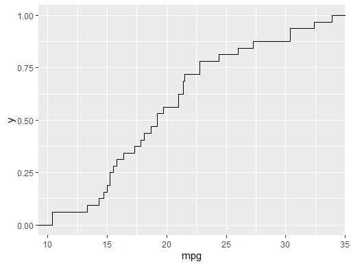
5.stat_ecdf()
stat_scdf()函数生成一个概率密度分布图。
1 | ggplot(mtcars,aes(mpg))+ |
6. stat_count()
state_identity(),表示映射值和data的值一样。
而stat_count()表示对data中的某个变量进行计数,stat_count()适用的几何形状:geom_point()、geom_bar()
例如,下面两个等价:
1 | ggplot(iris,aes(Species,after_stat(count)))+ |
1 | ggplot(iris,aes(Species,after_stat(count)))+ |
7. stat_density()
可以看做是直方图count计数的平滑版本。
适用几何形状:geom_area()、geom_line()、geom_point()、geom_density()。
1 | ggplot(iris,aes(Sepal.Length))+ |
1 | ggplot(iris,aes(Sepal.Length))+ |
1 | ggplot(iris,aes(Sepal.Length))+ |
1 | ggplot(iris,aes(Sepal.Length))+ |
8. stat_boxplot()
默认几何形状:boxplot()
适用几何形状:geom_boxplot()、geom_point()。
如下,boxplot()括号中的都可以省略。
1 | ggplot(iris,aes(Species,Sepal.Length))+ |
1 | ggplot(iris,aes(Species,Sepal.Length))+ |
9. stat_ydensity()
boxplot的密度图呈现。默认几何形状:geom_violin();
适用几何形状:geom_violin()、geom_point()。
1 | ggplot(iris,aes(Species,Sepal.Length))+ |
1 | ggplot(iris,aes(Species,Sepal.Length))+ |
10. stat_bindot()
适用几何形状:geom_dotplot()。
1 | ggplot(iris,aes(Sepal.Length))+ |
11. stat_bin_2d()
统计落在x和y区域(长方形)上点的个数。
适用几何形状:geom_tile()、geom_point()、geom_bin2d()。
1 | ggplot(iris,aes(Sepal.Length,Sepal.Width))+ |
12. stat_bin_hex()
stat_bin_2d的六边形版本。适用几何形状:geom_hex()。
1 | ggplot(iris,aes(Sepal.Length,Sepal.Width))+ |
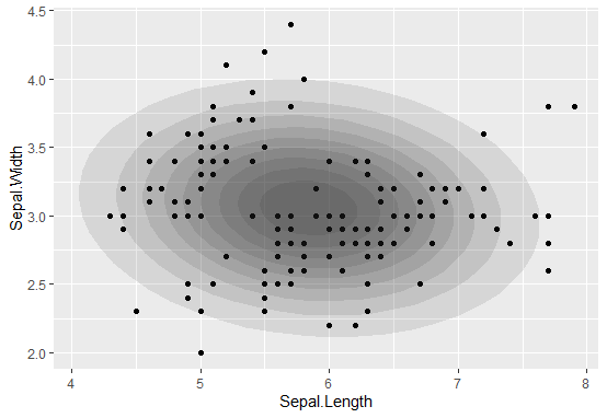
13. stat_density_2d()
二维核密度估计,二维版本的stat_density()。
适用几何形状:geom_density_2d()、geom_raster()、geom_tile()、geom_path()、geom_point()、geom_polygon()。
1 | ggplot(iris,aes(Sepal.Length,Sepal.Width))+ |
绘制出的图形为等高线。
14. stat_ellipse()
假定数据服从多元分布,计算椭圆图形需要的参数。
适用几何形状:geom_path()。
1 |
|
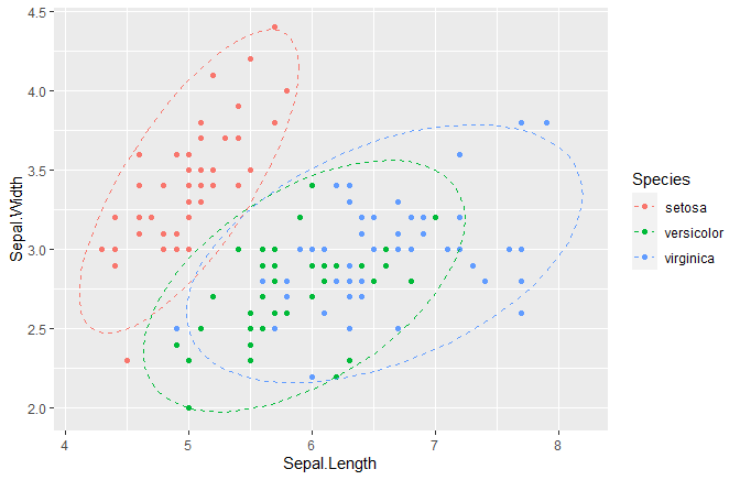
1 | iris %>% |
还有好多stat函数,如:stat_function()、stat_spoke()、stat_quantile()、stat_summary_2d()、stat_summary_hex()、stat_contour()、stat_contour_filled()。