本文总结一下ggplot2包绘图的一些基本图形语法。
1.ggplot2包的介绍
在ggplot2中,图是采用+号函数创建并串联起来的,每个函数修改属于自己的部分。例如:
1 | ggplot(data=mtcars, aes(x=wt,y=mpg))+ |
基本元素:
- 数据:作图用的数据集
- 几何图形 geom_:表示数据的几何形状,更多形状推荐这里
- 点图、折线图、箱线图、小提琴图等等
- 映射 aes(): 几何或者统计对象的映射
- x(x轴方向的位置)
- y(y轴方向的位置)
- color(点或者线等元素的颜色
- size(点或者线等元素的大小)
- shape(点或者线等元素的形状)
- alpha(点或者线等元素的透明度)
- 面 facet_: 数据图表的排列
- 标度 scale_(): 数据与美学维度之间的映射,比如图形宽度的数据范围
- 统计转换 stat_: 数据的统计,比如百分位,拟合曲线
- 坐标系统 coord_: 数据的转换
- 图层 layer:增加图层
- 主题 theme(): 图形的整体视觉默认值,如背景、网格、轴、默认字体、大小和颜色
ggplot默认至少需要前三样:数据、数据如何映射到美学aes()、几何图形geom_。
2. aes()
aes()函数是ggplot2中的映射函数, 所谓的映射即为数据集中的数据关联到相应的图形属性过程中一种对应关系。每个点都有自己图像上的属性,比如x坐标,y坐标,点的大小、颜色和形状,这些都叫做aesthetics,即图像上可观测到的属性,通过aes函数来赋值。
关于aes(),ggplot2解释如下:
The aes argument stands for aesthetics. ggplot2 considers the X and Y axis of the plot to be aesthetics as well, along with color, size, shape, fill etc. If you want to have the color, size etc fixed (i.e. not vary based on a variable from the dataframe), you need to specify it outside the aes(), like this.
即如果颜色是指定的,而不是根据数据值变化,那么需要将color参数下载aes()外面,如下:
1 | > ggplot(diamonds,aes(x=carat,color=color)) |
具体aes()如下图: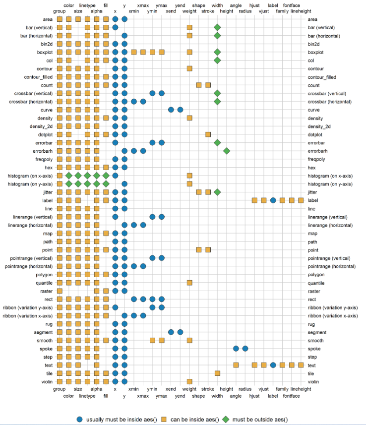
例如: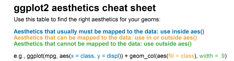
3. facet分面
分面设置在ggplot2应该也是要经常用到的一项画图内容,在数据对比以及分类显示上有着极为重要的作用。分组指的是在一个图形中显示两组或多组观察结果。 小面化指的是在单独、并排的图形上显示观察组。
facet_wrap和facet_grid不同在于facet_wrap是基于一个因子进行设置,facets表示形式为:~ 变量
而facet_grid是基于两个因子进行设置,facets表示形式为:变量 ~ 变量(行 ~ 列),如果把一个因子用点表示,也可以达到facet_wrap的效果,也可以用加号设置成两个以上变量
例如:变量+变量~变量 的形式,表示对三个变量设置分面。
3.1 facet_wrap()
1 | facet_wrap(facets, nrow = NULL, ncol = NULL, scales = "fixed", shrink = TRUE, as.table = TRUE, drop = TRUE) |
参数说明:
- nrow,ncol : 分面所设置成的行和列,参数为数值,表示几行或者几列
- scales : 参数fixed表示固定坐标轴刻度,free表示反馈坐标轴刻度,也可以单独设置成free_x或free_y(把scales 设置成free之后,可以看出每个分面都有自己的坐标刻度,当然我们也可以单独对x轴或y轴设置)
- shrink : 也和坐标轴刻度有关,如果为TRUE(默认值)则按统计后的数据调整刻度范围,否则按统计前的数据设定坐标
- drop : 表示是否去掉没有数据的分组,默认情况下不显示,逻辑值为FALSE
实例:
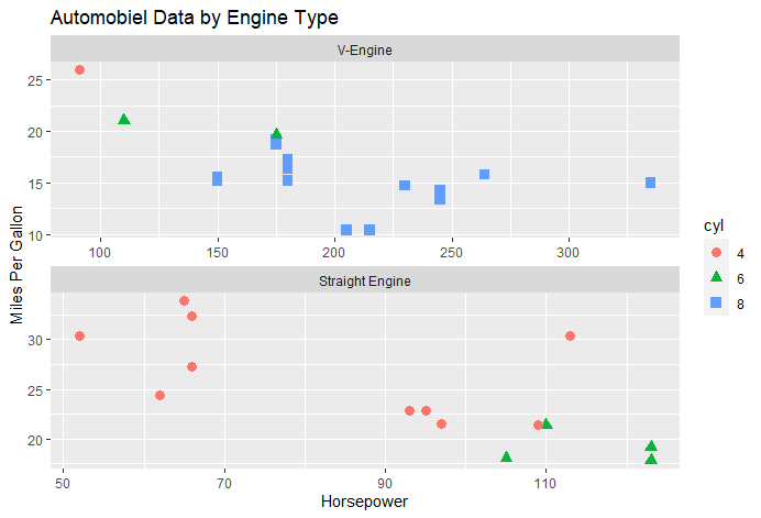
首先,将am、 vs和cyl变量转化为因子:
1 | mtcars$am <- factor(mtcars$am, levels=c(0,1), |
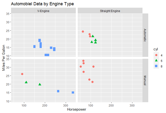
接下来,利用下面的代码绘图:
1 | ggplot(data=mtcars, aes(x=hp, y=mpg, shape=cyl, color=cyl)) + |
3.2 facet_grid()
1 | facet_grid(facets, margins = FALSE, scales = "fixed", space = "fixed", shrink = TRUE, labeller = "label_value", as.table = TRUE, drop = TRUE) |
参数说明:
- scales 、shrink、drop 同上
- as.table :和小图排列顺序有关的选项。如果为TRUE(默认)则按表格方式排列,即最大值(指分组level值)排在表格最后即右下角,否则排在左上角
- margins :通过TRUE或者FALSE表示否设置而一个总和的分面变量,默认情况为FALSE,即不设置
- space :表示分面空间是否可以按数据进行缩放,参数和scales一样
实例:
利用下面的代码绘图:
1 | library(ggplot2) |
4. 刻度 scale 相关设置
scale_主要用于在ggplot画图之后对各个图层进行调整。
4.1 相关属性设置
包括scale_size()、scale_alpha()、scale_shape()。这三个设置主要对ggplot的图层属性进行相关设置,包括尺寸、透明度和形状。
以下列出该设置的主要参数:
1 | scale_xxx(name = waiver(), breaks = waiver(), labels = waiver(), limits = NULL, range = c(1, 6),.....) |
由上面参数可以看出,我们可以对该属性进行,name命名,breaks设置组别,labels组别标签,limits限定坐标轴范围或组别排序,这几个参数在大多数scale设置中基本上都会用到。range设置尺寸大小范围(如点图的点),这个参数在其他设置中相对少见。
scale_size
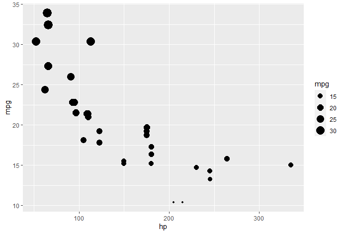
下面提供些例子作为参考:以R自带的mtcars数据集作为样本
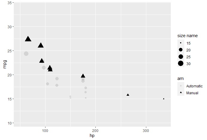
1 | ggplot(data=mtcars, aes(x=hp, y=mpg,size=mpg)) + |
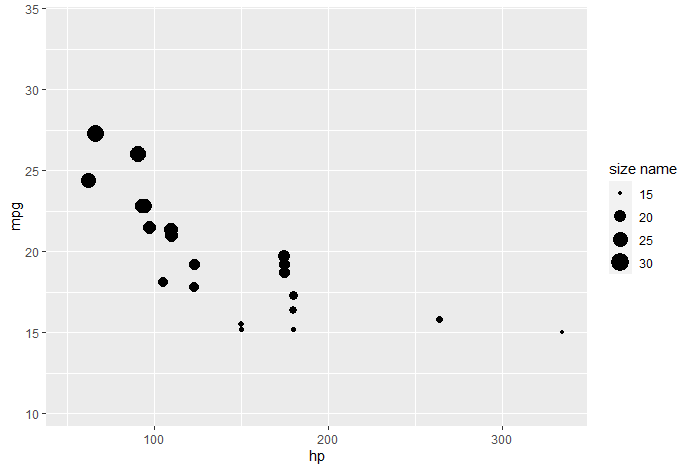
修改size的图例为”size name”,同时使用limits将size进行限定,只有在limits设置范围内的数据会被保留。
1 | ggplot(data=mtcars, aes(x=hp, y=mpg,size=mpg)) + |
range参数通过缩放修改点的大小。
1 | ggplot(data=mtcars, aes(x=hp, y=mpg,size=mpg)) + |
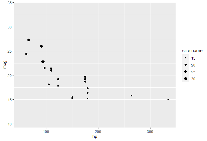
limits设置是针对数据的范围进行裁剪,而range设置纯粹的针对点的大小。scale_size()基本只用于散点图,同时与之对应的还有一个scale_radius()是对点进行设置半径,相比较而言scale_radius()基本上很少用到。最后scale_size诸多设置也可以用scale_size_area()进行设置。
scale_alpha
alpha调整点的透明度,scale_alpha与scale_alpha_continuous()等价,参数如下:
1 | scale_alpha(..., range = c(0.1, 1)) |
关于alpha参数的其他设置如name、breaks等归进continuous_scale()、binned_scale()、 discrete_scale()函数,区别在于alpha分组的变量是连续型(数值型)还是离散型(如文本类型)。
1 | continuous_scale( |
例如,连续型:
1 | ggplot(data=mtcars, aes(x=hp, y=mpg,size=mpg,alpha=mpg)) + |
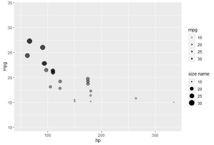
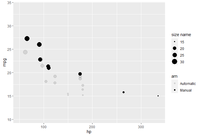
离散型:
1 | ggplot(data=mtcars, aes(x=hp, y=mpg,size=mpg,alpha=am)) + |
scale_shape
scale_shape只能用于离散型变量,例如:
1 | ggplot(data=mtcars, aes(x=hp, y=mpg,size=mpg,alpha=am,shape=am)) + |