RNA-seq分析(3)之DESeq2差异分析

利用DESeq2包进行差异表达分析。

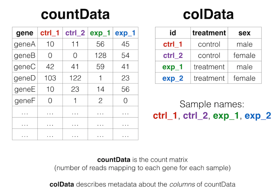
1. 读入数据并构建DESeq2对象

DESeq2差异分析是使用原始counts数据进行分析的，首先要创建DESeq2包能够处理的对象，创建该对象需要三个数据集：
countData基因计数矩阵:行为基因，列为每个样本。
colData样本信息数据：分别哪个样本是control、哪个是treatment。
group_list：分组信息。
这三个数据中的样本id要一致，否则会报错。
数据结构如图所示：

读入数据及预处理：

library(DESeq2)
library(dplyr)
library(ggplot2)
library(ggrepel)

# 读入数据
count <- read.table(file = "counts.txt")
# 命名行和列的名字:行名为第一列
rownames(count) <- count$V1
count <- count[,2:5]
count <- count[rowSums(count)>0,]
colnames(count) <- c("CS-1","CS-2","PS-1","PS-2")
count <- count[-1,]

三个dataframe：
ColData:样本和分组的对应信息,即colData；
grouplist:分组信息；
countData:rawcounts,即count。

group_list <- rep(c("CS","PS"),each =2)

colData <- data.frame(sample = colnames(count),
                      group_list = group_list )

有了这三个矩阵信息，就可以进行接下来DESeq2对象的构建了。

1 2	dds <- DESeqDataSetFromMatrix(countData = count,colData = colData, design = group_list)

2. 差异分析

接下来可以进行差异分析,并提取差异分析的结果。

1
2
3

dds2 <- DESeq(dds)
# 提取差异分析结果
res <- results(dds2,contrast=c("group_list","CS","PS"))

这里需要注意contrast参数，两个组的先后顺序如果不同分析出来的差异。原文是这样写的：

The results table when printed will provide the information about the comparison, e.g. “log2 fold change (MAP): condition treated vs untreated”, meaning that the estimates are of log2(treated / untreated), as would be returned by contrast=c(“condition”,”treated”,”untreated”).

所以两个组的顺序应该是对照在后面，实验组在前面，否则得到的上下调基因会刚好相反。

res中包含的列：base means across samples, log2 fold changes, standard errors, test statistics, p-values and adjusted p-values。
由于我的gene id用的是果蝇flybase数据库中的id，所以我希望在得到的结果中添加上gene symbol信息用于火山图部分基因的标记，添加entrez id以便后续的kegg分析。

res$symbol <- mapIds(org.Dm.eg.db, 
                     keys=row.names(res), 
                     column="SYMBOL", 
                     keytype="ENSEMBL",
                     multiVals="first")
res$entrez <- mapIds(org.Dm.eg.db, 
                     keys=row.names(res), 
                     column="ENTREZID", 
                     keytype="ENSEMBL",
                     multiVals="first")
res$name =   mapIds(org.Dm.eg.db,
                    keys=row.names(res), 
                    column="GENENAME",
                    keytype="ENSEMBL",
                    multiVals="first")

# 按照pvalue大小排序
res_ordered <- res[order(res$pvalue),]

DEG <- as.data.frame(res_ordered)
# 去除NA值：na.omit()去除含有NA值的整行数据
DEG <- na.omit(DEG)

3. 根据差异表达倍数确定上下调的基因

确定上下调表达的基因，可以选择静态阈值或者动态阈值。静态阈值比如：p<0.05,logFC>2。动态阈值根据数据整体的情况确定一个阈值。

如果采用动态阈值，则计算动态阈值的代码如下：

1
2
3

# 动态阈值计算：差异倍数绝对值的均值±两倍标准差
logFC_t <- with(DEG,mean(abs(log2FoldChange)) + 2*sd(abs(log2FoldChange)))
logFC_t <- round(logFC_t, 2) #取前两位小数

这里以采用静态阈值2为例进行分析并绘制火山图，也可以采用padj确定上下调基因。

DEG$change = as.factor(ifelse(DEG$pvalue < 0.05 & abs(DEG$log2FoldChange) > 2,
                              ifelse(DEG$log2FoldChange > 2 ,'UP','DOWN'),'STABLE'))
table(DEG$change)

DEG$label <- ifelse(DEG$pvalue < 0.00000001 & abs(DEG$log2FoldChange) >= 3,
                    DEG$symbol,"")

ggplot(DEG, aes(x=log2FoldChange, y=-log10(pvalue),color=change)) + 
  geom_point(alpha=0.4, size=2) + 
  theme_classic() + 
  xlab("log2 fold change") +
  ylab("-log10 pvalue") +
  theme(plot.title = element_text(size=15,hjust = 0.5)) + 
  scale_colour_manual(values = c('blue','black','red')) +
  geom_hline(yintercept = -log10(0.05), lty = 2) +
  geom_vline(xintercept = c(-2, 2), lty = 2) +
  geom_label_repel(data = DEG, aes(label = label),
                   size = 3,box.padding = unit(0.5, "lines"),
                   point.padding = unit(0.8, "lines"),
                   segment.color = "black",
                   show.legend = FALSE, max.overlaps = 10000)

到这里，差异分析就完成啦！

参考链接：